Methods that we used to explore the effect of missingness on fairness

Replicating Each Type of Missingness

MCAR: Missing Completely at Random

In order to replicate this type of missingness, our mcar function simply takes in a user-input probability parameter, which designates how likely each value in the attribute is to be missing. This is the simplest form of missingness to reproduce, since missingness is completely at random and not dependent on any particular value. Therefore, we can just set a threhold and for each tuple, generate a random value between 1 and 100. If the generated value is less than or equal to the threshold, the tuple's value can be set to missing, and it remains its original value otherwise. This happens for each tuple for the selected attribute.

NMAR: Not Missing at Random

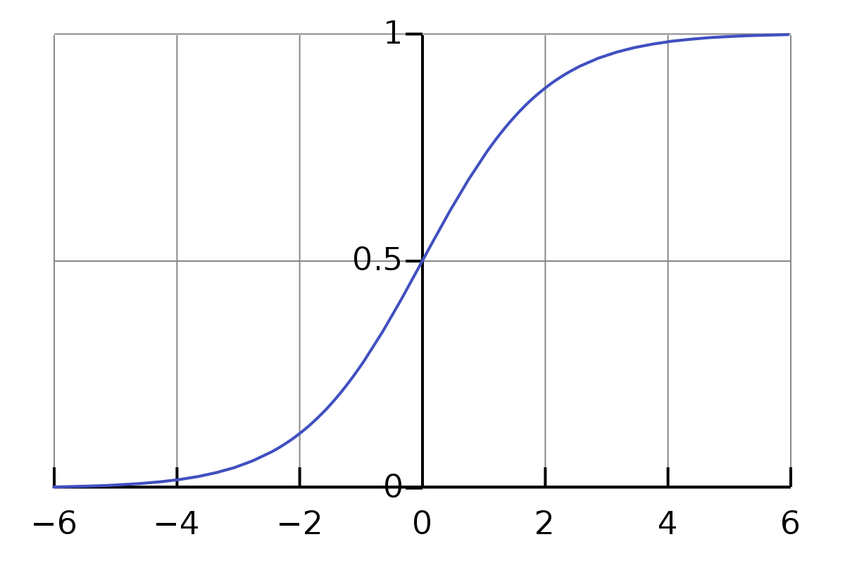
In order to generate our NMAR data, we make use of sigmoid function. This is because the sigmoid function conviniently produces a value between 0 and 1 (and therefore can be interpreted as a probability).

What happens before this is dependent on the type of the attribute in which missingness will be generated. If the column is categorical, for each unique categorical value, a random z-score is generated from a normal distribution and put into a sigmoid function. This will produce a probability for each unique value of the column. If the column is numerical, the z-score of each value is determined and passed into a sigmoid function to determine the probability of missingness for each value. Whether each value in the column will be missing is determined by th probability generated by the sigmoid function, using a threshold as explained previously. The beta value is multiplied by the generated probability as a way to tune how much missingness is generated. The higher the beta value (between 0 and 1), the more missingness is generated.

MAR: Missing at Random

Our MAR data is generated in a very similar way to our NMAR data. The only difference is that the value of the column that our attribute is dependent on is used rather than the value of the missingness column itself.

Fairness Notions

Statistical Parity

Statistical parity occurs when the following equation is satisfied:
P (R = +|A = a) = P (R = +|A = b)∀a, b ∈ A
where A is the set of sensitive characteristics and R is the predictive outcome. In a perfectly fair algorithm, the two sides of the equation are equal; therefore, the closest we get the difference between P (R = +|A = a) and P (R = +|A = b) to 0, the better our intervention technique is at improving fairness.

Equality of Opportunity

Equality of Opportunity allows for individuals within the "advantaged" group to be given an equal chance of correctly classified. In other words, we want the True Positive Rate to be equal for every attribute in the protected class. Equality of opportunity is a type of fairness where each sample, model should be treated similarly, with no bias or preference, except where particular distinctions can be explicitly justified.

Equality of Odds

Equality of Odds is a much stricter version of equality of opportunity. Instead of using True Positive Rate to be equal in every attributes, it rather takes in the lowest False Negative Rate and uses them as the guide to make all the rates equal in all of the attributes.

Fairness Intervention Technique(s)

Adversarial Debiasing (Inprocessing)

In adversarial debiasing, two models are built within the method. The first is predicting the target label. The second model is the adversary, which tries to predict, based on the predictions of the first model, what the sensitive attribute is for each tuple. Ideally, this adversarial model shouldn't be able to predict it well. Next, the adversarial model makes modifications to the original model with parameters and weighting that weaken the predictive power of the adversarial model until it cannot predict the protected attributes well.